DIRESA tutorial
1. Install packages
The diresa-torch package depends on the PyTorch package. This tutorial also uses numpy and matplotlib.
[1]:
# Install needed packages
!pip install numpy
!pip install matplotlib
!pip install diresa-torch
Requirement already satisfied: diresa-torch in /usr/local/lib/python3.12/dist-packages (1.0.0)
2. Load the dataset
In this tutorial, we are going to compress the 3D lorenz ‘63 butterfly into a 2D latent space. The lorenz.csv contains a list of butterfly points, with three colums for the X, Y and Z coordinate.
[2]:
!wget https://gitlab.com/etrovub/ai4wcm/public/diresa/-/raw/master/docs/lorenz.csv
--2025-09-24 08:00:58--  https://gitlab.com/etrovub/ai4wcm/public/diresa/-/raw/master/docs/lorenz.csv
Resolving gitlab.com (gitlab.com)... 172.65.251.78, 2606:4700:90:0:f22e:fbec:5bed:a9b9
Connecting to gitlab.com (gitlab.com)|172.65.251.78|:443... connected.
HTTP request sent, awaiting response... 200 OK
Length: 2999999 (2.9M) [text/plain]
Saving to: ‘lorenz.csv.8’

lorenz.csv.8        100%[===================>]   2.86M  --.-KB/s    in 0.02s

2025-09-24 08:00:59 (133 MB/s) - ‘lorenz.csv.8’ saved [2999999/2999999]
[3]:
import numpy as np
data_file = "lorenz.csv"
data = np.loadtxt(data_file, delimiter=",").astype(np.float32)
print("Shape", data_file, ":", data.shape)
train = data[:30000]
val = data[30000:35000]
test = data[35000:]
Shape lorenz.csv : (40000, 3)
3. Build the DIRESA model
We can build a DIRESA model with convolutional and/or dense layers with the Diresa.from_hyper_param class method. We can also build a DIRESA model based on a custom encoder and decoder with the Diresa.from_custom class method (see below). We build a model with an input shape of (3,) for the 3D butterfly points. Our encoder model has 3 dense layers with 40, 20 and 2 units (the latter is the dimension of the latent space). The decoder is a reflection of the encoder.
[4]:
import torch.nn as nn
from diresa_torch.arch.models import Diresa

diresa = Diresa.from_hyper_param(input_shape=(3, ), dense_units=(40, 20, 2), activation=nn.ReLU())
print(diresa)
Diresa(
  (base_encoder): Encoder(
    (network): DenseLayer(
      (network): Sequential(
        (0): Linear(in_features=3, out_features=40, bias=True)
        (1): ReLU()
        (2): Linear(in_features=40, out_features=20, bias=True)
        (3): ReLU()
        (4): Linear(in_features=20, out_features=2, bias=True)
      )
    )
  )
  (dist_layer): DistanceLayer()
  (base_decoder): Decoder(
    (network): DenseLayer(
      (network): Sequential(
        (0): Linear(in_features=2, out_features=20, bias=True)
        (1): ReLU()
        (2): Linear(in_features=20, out_features=40, bias=True)
        (3): ReLU()
        (4): Linear(in_features=40, out_features=3, bias=True)
      )
    )
  )
  (ordering_layer): OrderingLayer()
)
4. Train the DIRESA model
We train the DIRESA model with the train_diresa function. The parameters include i.a. the diresa model, the dataloaders and the 3 loss functions with their weights. The DIRESA model has 3 loss functions, the reconstruction loss (usually the MSE is used here), the covariance loss and a distance loss (here the MSE distance loss is used). The batch size must be large enough for the calculation of the covariance loss, which calculates the covariance matrix of the latent space components over the
batch. A shuffled version of the batches is fed in the twin encoder for calculating the distance loss (so also for this one, the batch size must be large enough). If staged_training is True, the encoder and decoder are trained separately.
[5]:
from torch.optim import Adam
from torch.cuda import is_available
from torch.utils.data import DataLoader
from diresa_torch.training.trainer import train_diresa
from diresa_torch.losses.loss_funcs import MSEDistLoss, LatentCovLoss
import logging

logging.basicConfig(level=logging.INFO, force = True)

device = "cuda" if is_available() else "cpu"
diresa = diresa.to(device)

hist = train_diresa(model=diresa,
                   train_loader=DataLoader(train, batch_size=512, shuffle=True),
                   #val_loader=DataLoader(val, batch_size=512, shuffle=True),
                   criteria=[nn.MSELoss(), LatentCovLoss(), MSEDistLoss()],
                   loss_weights=[1., 1., 1.],
                   optimizer=Adam(diresa.parameters(), lr=0.001),
                   num_epochs=10,
                   staged_training=False,
                   )
INFO:root:Encoder_Decoder: Epoch 1/10 - ReconMSELoss_train: 1.1770e-01, LatentCovLoss_train: 5.5410e-08, MSEDistLoss_train: 1.0775e-05, WeightedLoss_train: 1.1771e-01
INFO:root:Encoder_Decoder: Epoch 2/10 - ReconMSELoss_train: 4.2598e-02, LatentCovLoss_train: 1.9488e-05, MSEDistLoss_train: 8.3505e-06, WeightedLoss_train: 4.2626e-02
INFO:root:Encoder_Decoder: Epoch 3/10 - ReconMSELoss_train: 1.9493e-02, LatentCovLoss_train: 4.8181e-04, MSEDistLoss_train: 1.7763e-06, WeightedLoss_train: 1.9977e-02
INFO:root:Encoder_Decoder: Epoch 4/10 - ReconMSELoss_train: 2.0258e-03, LatentCovLoss_train: 6.7263e-05, MSEDistLoss_train: 8.8855e-07, WeightedLoss_train: 2.0939e-03
INFO:root:Encoder_Decoder: Epoch 5/10 - ReconMSELoss_train: 1.0372e-03, LatentCovLoss_train: 6.0002e-05, MSEDistLoss_train: 1.0330e-06, WeightedLoss_train: 1.0982e-03
INFO:root:Encoder_Decoder: Epoch 6/10 - ReconMSELoss_train: 8.3148e-04, LatentCovLoss_train: 6.7772e-05, MSEDistLoss_train: 9.6441e-07, WeightedLoss_train: 9.0022e-04
INFO:root:Encoder_Decoder: Epoch 7/10 - ReconMSELoss_train: 7.0734e-04, LatentCovLoss_train: 7.6553e-05, MSEDistLoss_train: 8.2719e-07, WeightedLoss_train: 7.8472e-04
INFO:root:Encoder_Decoder: Epoch 8/10 - ReconMSELoss_train: 6.2208e-04, LatentCovLoss_train: 4.6304e-05, MSEDistLoss_train: 7.0290e-07, WeightedLoss_train: 6.6909e-04
INFO:root:Encoder_Decoder: Epoch 9/10 - ReconMSELoss_train: 5.4353e-04, LatentCovLoss_train: 5.2800e-05, MSEDistLoss_train: 6.2335e-07, WeightedLoss_train: 5.9695e-04
INFO:root:Encoder_Decoder: Epoch 10/10 - ReconMSELoss_train: 4.6981e-04, LatentCovLoss_train: 4.3592e-05, MSEDistLoss_train: 5.4320e-07, WeightedLoss_train: 5.1395e-04
5. Evaluate the DIRESA model
We evaluate the DIRESA model with the evaluate_diresa function. The bigger the batch size, the more accurate the covariance and distance losses will be.
[6]:
from diresa_torch.training.trainer import evaluate_diresa

hist = evaluate_diresa(model=diresa,
                       test_loader=DataLoader(test, batch_size=5000),
                       criteria=[nn.MSELoss(), LatentCovLoss(), MSEDistLoss()],
                       loss_weights=[1., 1., 1.],
                       )
INFO:root:ReconMSELoss_eval: 5.1149e-04, LatentCovLoss_eval: 8.1919e-06, MSEDistLoss_eval: 5.5916e-09, WeightedLoss_eval: 5.1969e-04
6. Order the latent components
The ordering of the latent components is done by calculating the R2 values for each of them for a given dataset. This is done with the order_diresa function. Again, the bigger the batch size, the more accurate the R2 calculation will be.
[7]:
from diresa_torch.training.trainer import order_diresa

order_diresa(model=diresa, data_loader=DataLoader(test, batch_size=5000))
INFO:root:Batch size for ordering is 5000
INFO:root:Ordered R2 scores are: [0.5434688329696655, 0.41254401206970215]
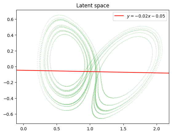
7. Show latent space
We plot the 2D latent space. As we ordered the latent components, the biggest variance should be in the x-axes direction.
[8]:
import matplotlib.pyplot as plt
from torch import from_numpy

latent = diresa.encode(from_numpy(test).to(device)).cpu().detach().numpy()
plt.figure()
plt.title("Latent space")
plt.scatter(latent[:, 0], latent[:, 1], marker='.', s=0.1, color='C2')
m, b = np.polyfit(latent[:, 0], latent[:, 1], deg=1)
plt.axline(xy1=(0, b), slope=m, color='r', label=f'$y = {m:.2f}x {b:+.2f}$')
plt.legend()
plt.show()
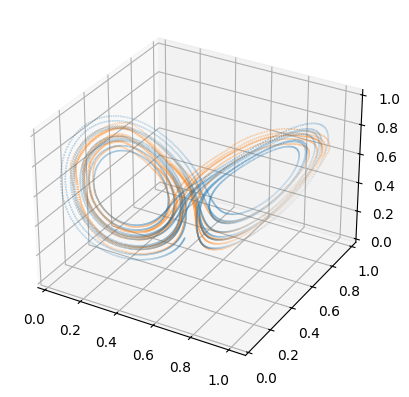
8. Original versus decoded datset
We compair the origonal dataset with the decoded one.
[9]:
predict = diresa.decode(from_numpy(latent).to(device)).cpu().detach().numpy()

fig = plt.figure()
ax = fig.add_subplot(projection='3d')
ax.scatter(val[:, 0], val[:, 1], val[:, 2], marker='.', s=0.1)
ax.scatter(predict[:, 0], predict[:, 1], predict[:, 2], marker='.', s=0.1, color='C1')
plt.show()
9. A convolutional example
If your dataset consists of a number of variables (e.g. temperature and pressure, so 2 variables) over a 2 dimensional grid, convolutional layers can be used in the encoder/decoder. Here is an example for a grid (y, x) = (32, 64). The dataset would then have a shape of (nbr_of_samples, 2, 32, 64). We will use a stack of 3 convolutional/maxpooling blocks in the encoder (the decoder mirrors the encoder). The first block uses 3 Conv2D layers, the second bock 2 and the third block 1, followed by a MaxPooling2D layer (stack=(3, 2, 1)). The number of filters in the first block is 32, in the second 16 and in the third 8 (stack_filters=(32, 16, 8)).
[10]:
diresa_conv = Diresa.from_hyper_param(input_shape=(2, 32, 64),
                                      stack=(3, 2, 1),
                                      stack_filters=(32, 16, 8),
                                      )
print(diresa_conv)
Diresa(
  (base_encoder): Encoder(
    (cnn): CNNLayer(
      (cnn): Sequential(
        (0): _CNNBlock(
          (block): Sequential(
            (0): Conv2d(2, 32, kernel_size=(3, 3), stride=(1, 1), padding=(1, 1))
            (1): ReLU()
            (2): Conv2d(32, 32, kernel_size=(3, 3), stride=(1, 1), padding=(1, 1))
            (3): ReLU()
            (4): Conv2d(32, 32, kernel_size=(3, 3), stride=(1, 1), padding=(1, 1))
            (5): ReLU()
            (6): MaxPool2d(kernel_size=(2, 2), stride=(2, 2), padding=0, dilation=1, ceil_mode=False)
          )
        )
        (1): _CNNBlock(
          (block): Sequential(
            (0): Conv2d(32, 16, kernel_size=(3, 3), stride=(1, 1), padding=(1, 1))
            (1): ReLU()
            (2): Conv2d(16, 16, kernel_size=(3, 3), stride=(1, 1), padding=(1, 1))
            (3): ReLU()
            (4): MaxPool2d(kernel_size=(2, 2), stride=(2, 2), padding=0, dilation=1, ceil_mode=False)
          )
        )
        (2): _CNNBlock(
          (block): Sequential(
            (0): Conv2d(16, 8, kernel_size=(3, 3), stride=(1, 1), padding=(1, 1))
            (1): ReLU()
            (2): MaxPool2d(kernel_size=(2, 2), stride=(2, 2), padding=0, dilation=1, ceil_mode=False)
          )
        )
      )
    )
    (flatten): Flatten(start_dim=1, end_dim=-1)
    (network): Sequential(
      (0): CNNLayer(
        (cnn): Sequential(
          (0): _CNNBlock(
            (block): Sequential(
              (0): Conv2d(2, 32, kernel_size=(3, 3), stride=(1, 1), padding=(1, 1))
              (1): ReLU()
              (2): Conv2d(32, 32, kernel_size=(3, 3), stride=(1, 1), padding=(1, 1))
              (3): ReLU()
              (4): Conv2d(32, 32, kernel_size=(3, 3), stride=(1, 1), padding=(1, 1))
              (5): ReLU()
              (6): MaxPool2d(kernel_size=(2, 2), stride=(2, 2), padding=0, dilation=1, ceil_mode=False)
            )
          )
          (1): _CNNBlock(
            (block): Sequential(
              (0): Conv2d(32, 16, kernel_size=(3, 3), stride=(1, 1), padding=(1, 1))
              (1): ReLU()
              (2): Conv2d(16, 16, kernel_size=(3, 3), stride=(1, 1), padding=(1, 1))
              (3): ReLU()
              (4): MaxPool2d(kernel_size=(2, 2), stride=(2, 2), padding=0, dilation=1, ceil_mode=False)
            )
          )
          (2): _CNNBlock(
            (block): Sequential(
              (0): Conv2d(16, 8, kernel_size=(3, 3), stride=(1, 1), padding=(1, 1))
              (1): ReLU()
              (2): MaxPool2d(kernel_size=(2, 2), stride=(2, 2), padding=0, dilation=1, ceil_mode=False)
            )
          )
        )
      )
      (1): Flatten(start_dim=1, end_dim=-1)
    )
  )
  (dist_layer): DistanceLayer()
  (base_decoder): Decoder(
    (unflatten): Unflatten(dim=1, unflattened_size=(8, 4, 8))
    (cnn): CNNLayer(
      (cnn): Sequential(
        (0): _CNNTransposeBlock(
          (block): Sequential(
            (0): Upsample(scale_factor=2.0, mode='nearest')
            (1): ConvTranspose2d(8, 16, kernel_size=(3, 3), stride=(1, 1), padding=(1, 1))
            (2): ReLU()
          )
        )
        (1): _CNNTransposeBlock(
          (block): Sequential(
            (0): Upsample(scale_factor=2.0, mode='nearest')
            (1): ConvTranspose2d(16, 16, kernel_size=(3, 3), stride=(1, 1), padding=(1, 1))
            (2): ReLU()
            (3): ConvTranspose2d(16, 32, kernel_size=(3, 3), stride=(1, 1), padding=(1, 1))
            (4): ReLU()
          )
        )
        (2): _CNNTransposeBlock(
          (block): Sequential(
            (0): Upsample(scale_factor=2.0, mode='nearest')
            (1): ConvTranspose2d(32, 32, kernel_size=(3, 3), stride=(1, 1), padding=(1, 1))
            (2): ReLU()
            (3): ConvTranspose2d(32, 32, kernel_size=(3, 3), stride=(1, 1), padding=(1, 1))
            (4): ReLU()
            (5): ConvTranspose2d(32, 2, kernel_size=(3, 3), stride=(1, 1), padding=(1, 1))
            (6): ReLU()
          )
        )
      )
    )
    (network): Sequential(
      (0): Unflatten(dim=1, unflattened_size=(8, 4, 8))
      (1): CNNLayer(
        (cnn): Sequential(
          (0): _CNNTransposeBlock(
            (block): Sequential(
              (0): Upsample(scale_factor=2.0, mode='nearest')
              (1): ConvTranspose2d(8, 16, kernel_size=(3, 3), stride=(1, 1), padding=(1, 1))
              (2): ReLU()
            )
          )
          (1): _CNNTransposeBlock(
            (block): Sequential(
              (0): Upsample(scale_factor=2.0, mode='nearest')
              (1): ConvTranspose2d(16, 16, kernel_size=(3, 3), stride=(1, 1), padding=(1, 1))
              (2): ReLU()
              (3): ConvTranspose2d(16, 32, kernel_size=(3, 3), stride=(1, 1), padding=(1, 1))
              (4): ReLU()
            )
          )
          (2): _CNNTransposeBlock(
            (block): Sequential(
              (0): Upsample(scale_factor=2.0, mode='nearest')
              (1): ConvTranspose2d(32, 32, kernel_size=(3, 3), stride=(1, 1), padding=(1, 1))
              (2): ReLU()
              (3): ConvTranspose2d(32, 32, kernel_size=(3, 3), stride=(1, 1), padding=(1, 1))
              (4): ReLU()
              (5): ConvTranspose2d(32, 2, kernel_size=(3, 3), stride=(1, 1), padding=(1, 1))
              (6): ReLU()
            )
          )
        )
      )
    )
  )
  (ordering_layer): OrderingLayer()
)
10. Build DIRESA with custom encoder and decoder
We can also build DIRESA models with custom encoder and decoder (reconstruction) models. To show the API, we use the encoder and decoder of the previous model to create a DIRESA model.
[11]:
diresa_custom = Diresa.from_custom(diresa.base_encoder, diresa.base_decoder)
print(diresa_custom)
Diresa(
  (base_encoder): Encoder(
    (network): DenseLayer(
      (network): Sequential(
        (0): Linear(in_features=3, out_features=40, bias=True)
        (1): ReLU()
        (2): Linear(in_features=40, out_features=20, bias=True)
        (3): ReLU()
        (4): Linear(in_features=20, out_features=2, bias=True)
      )
    )
  )
  (dist_layer): DistanceLayer()
  (base_decoder): Decoder(
    (network): DenseLayer(
      (network): Sequential(
        (0): Linear(in_features=2, out_features=20, bias=True)
        (1): ReLU()
        (2): Linear(in_features=20, out_features=40, bias=True)
        (3): ReLU()
        (4): Linear(in_features=40, out_features=3, bias=True)
      )
    )
  )
  (ordering_layer): OrderingLayer()
)